Breaking Down the Jelly Slider

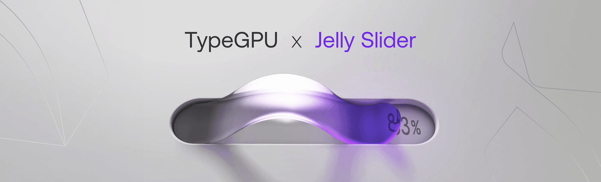
After the Jelly Slider implementation gained a lot of attention, I decided to write this post to explain how it works in detail and show you how to recreate it yourself, or even build your own visualization inspired by it.

We’ll explore how the simulation functions and how it’s rendered to the screen using only TypeScript with the help of TypeGPU. I’ll walk through the reasoning behind my decisions and share some insights into the trade-offs made along the way. Of course, there’s always room for further improvements and optimizations — it all comes down to the balance between time and effort.

Disclaimer: This is not a step by step implementation tutorial. I will focus primarily on explaining the methodology and will occasionally include snippets from the original code, which you can find in its entirety on the TypeGPU examples page or directly in the GitHub repository. Some snippets may be simplified or modified to avoid overwhelming the reader with code. You are free to reference the original implementation at any time, as the function names are kept intact.

The Simulation

The actual physical simulation happens in two-dimensional space, which greatly simplifies the amount of work we have to do. The implementation supports an arbitrary number of points but is empirically tuned to work with 17, which provides a good balance between performance and visual complexity.

The overall structure of the simulation is quite well represented by the code itself:

update(dt: number) {
  for (let s = 0; s < this.substeps; s++) {
    this.#integrate(h, damp, compression);
    this.#projectConstraints();
  }

  this.#computeNormals();
  this.#computeControlPoints();
  this.#updateGPUBuffer();
  this.#computeBezierPipeline.dispatchThreads(...BEZIER_TEXTURE_SIZE);
}

Where:

• h is the duration of a sub-step
• damp is a constant that represents additional resistance to movement
• compression is a normalized value that represents how far apart the ends are

Let’s go over the process step by step.

Integration

The main method used for calculating point positions is Verlet integration, which — despite its intimidating name — is actually very simple. We can think of it this way: if a point was previously at position A and is now at position B, its velocity corresponds to the vector from A to B.

Verlet integration updates each point’s position using its current and previous states, without explicitly storing velocity. The next position is estimated from the previous two, with some adjustments applied over time. In this case, there’s no gravity — instead, the middle section of the slider is slightly lifted to fit a sine-like curve when compressed.

Constraint projection

As mentioned earlier, the integration relies on the current position, previous position, and small adjustments over time. Apart from applying a varying arching force, we also need to enforce certain constraints. If we only applied the force, the points would drift away, and the result wouldn’t look stable.

To keep the simulation in shape, after each iteration we project constraints. In our case, those constraints are:

• the first point should stay fixed at its initial position
• the last point (handle) should stay fixed where the cursor is
• the distance between neighboring points should remain constant
• points near the ends should resist bending

They are enforced in two ways. The first two are hard constraints — we simply set the positions directly. The last two use distance projection. For the distance constraint, we measure the actual distance between two points and move each halfway toward their ideal separation. After several iterations, all segments are nearly at their correct lengths.

For bending resistance, the principle is similar, but instead of connecting two actual points equally, we compare a point to where a corresponding position along the y-axis would be, applying a smaller correction. In practice, this means we pull the endpoints back toward a straight line, but only partially.

These operations are enough for us to know where the slider is, but we still need to compute some additional data useful for rendering — specifically, the normals and control points.

Computing Normals

You can think of normals as the relative “up” directions at each point. They’re useful in many contexts — most commonly for calculating how light reflects off a surface during rendering. In our case, we won’t use them directly for the simulation (for reasons we’ll cover later), but they’re still important when we approximate the curvature of the slider.

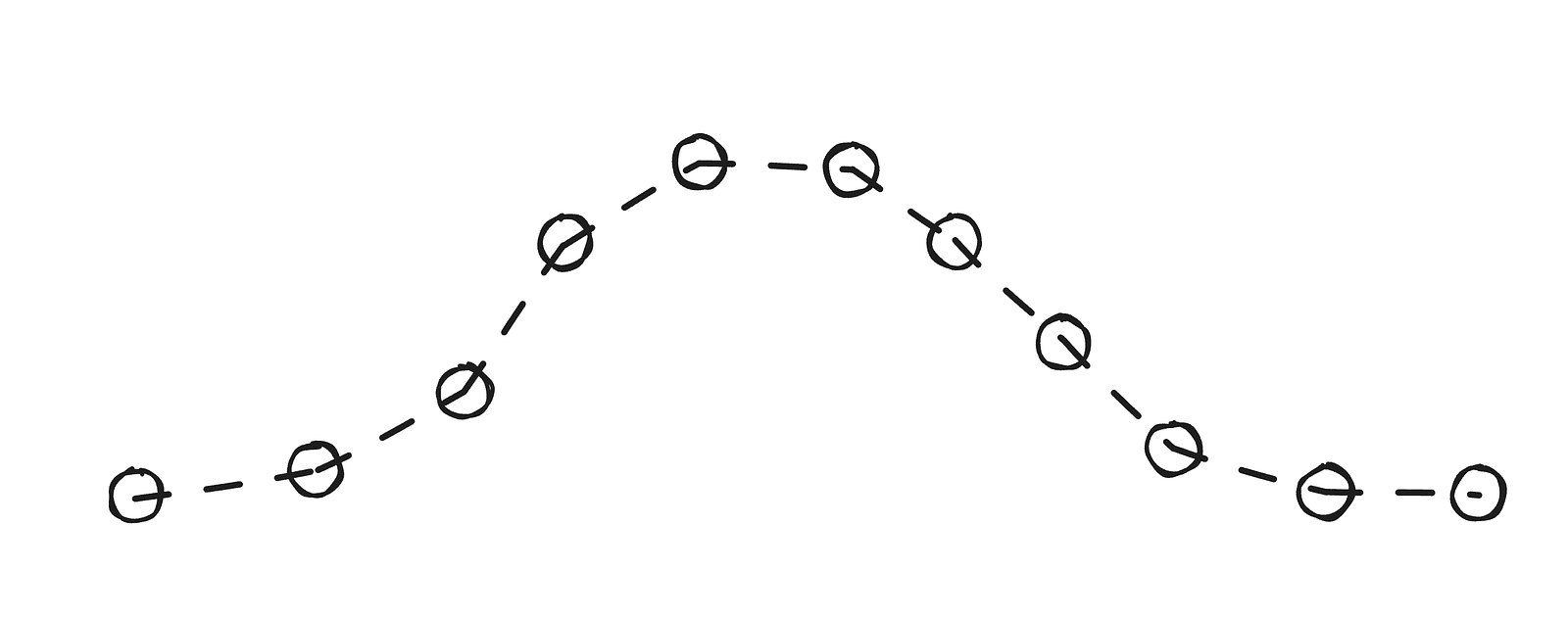
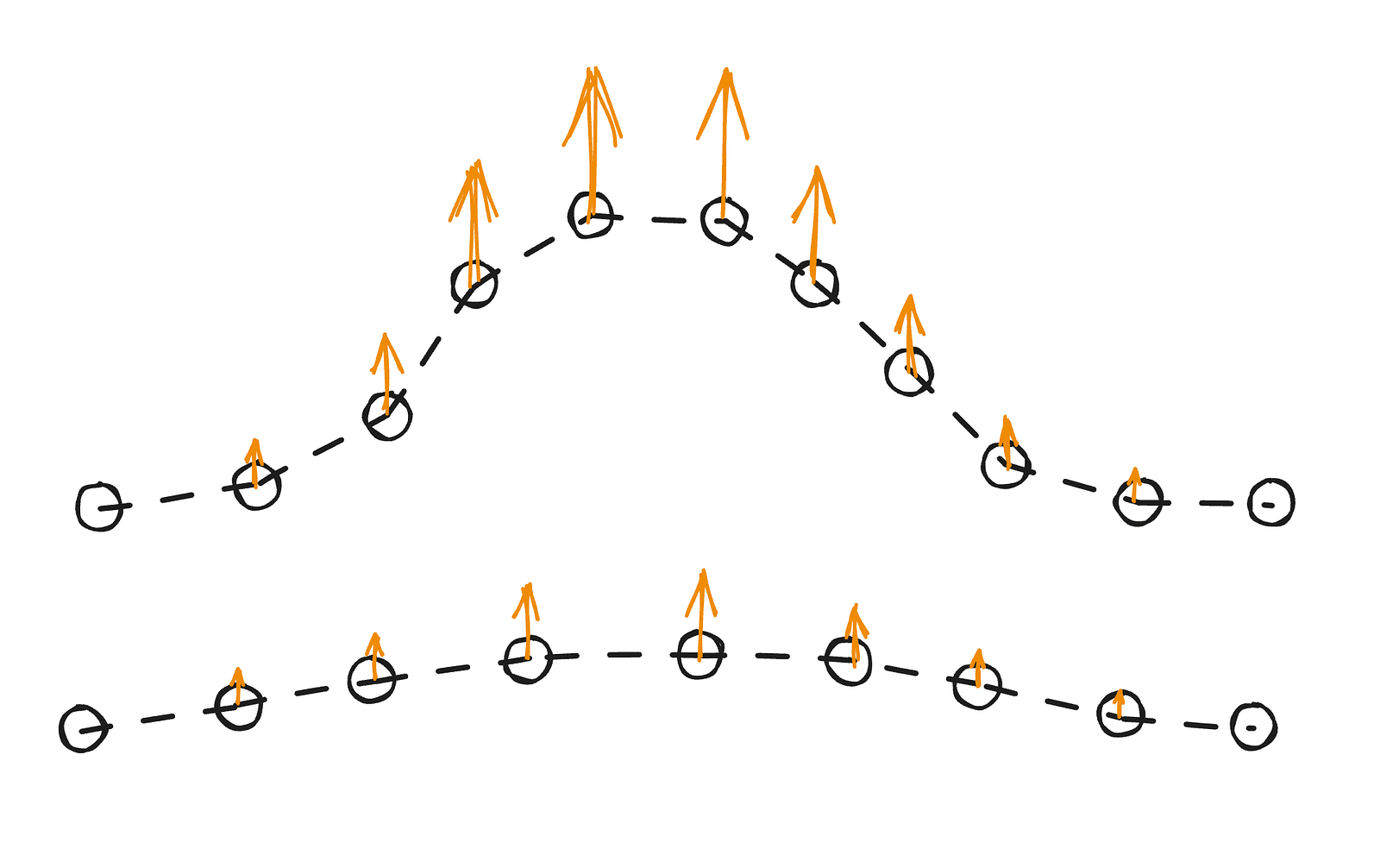
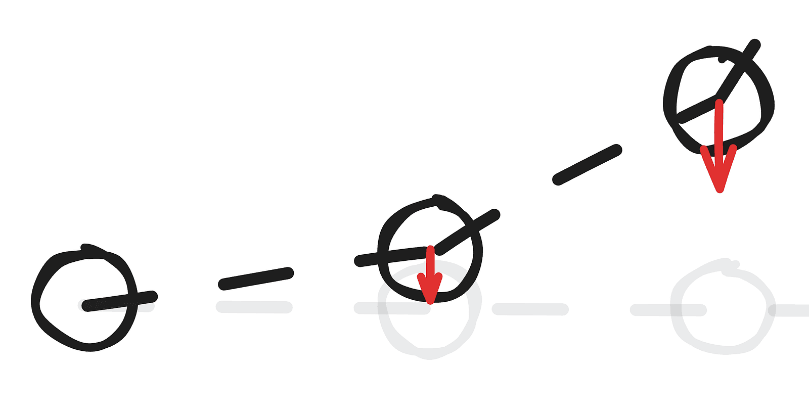
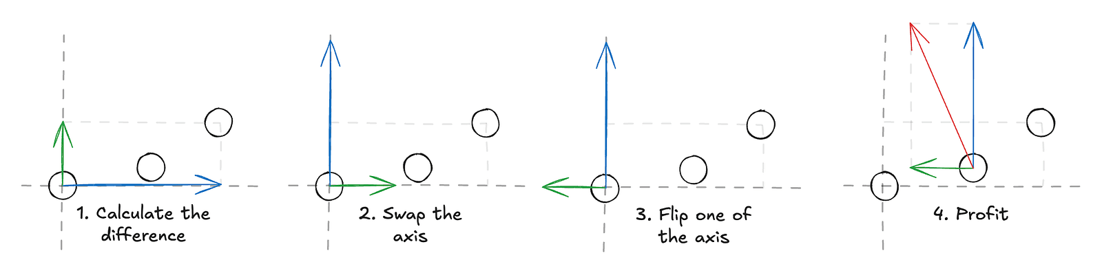
Calculating normals using three points is straightforward: we take the line defined by connecting the previous and next points and then compute a vector that’s perpendicular to it. For the edge cases — the first and last points — we can simply assume the normal points straight up.

Computing Control Points

The last piece of information we need before rendering relates to how we want to represent the slider. There are several options, but the approach I chose is to model it as a series of quadratic Bézier segments. This choice works well for two main reasons:

1. A quadratic Bézier curve is defined by just three points.
2. They can be easily represented as SDFs (signed distance fields — we’ll cover what those are in the rendering section).

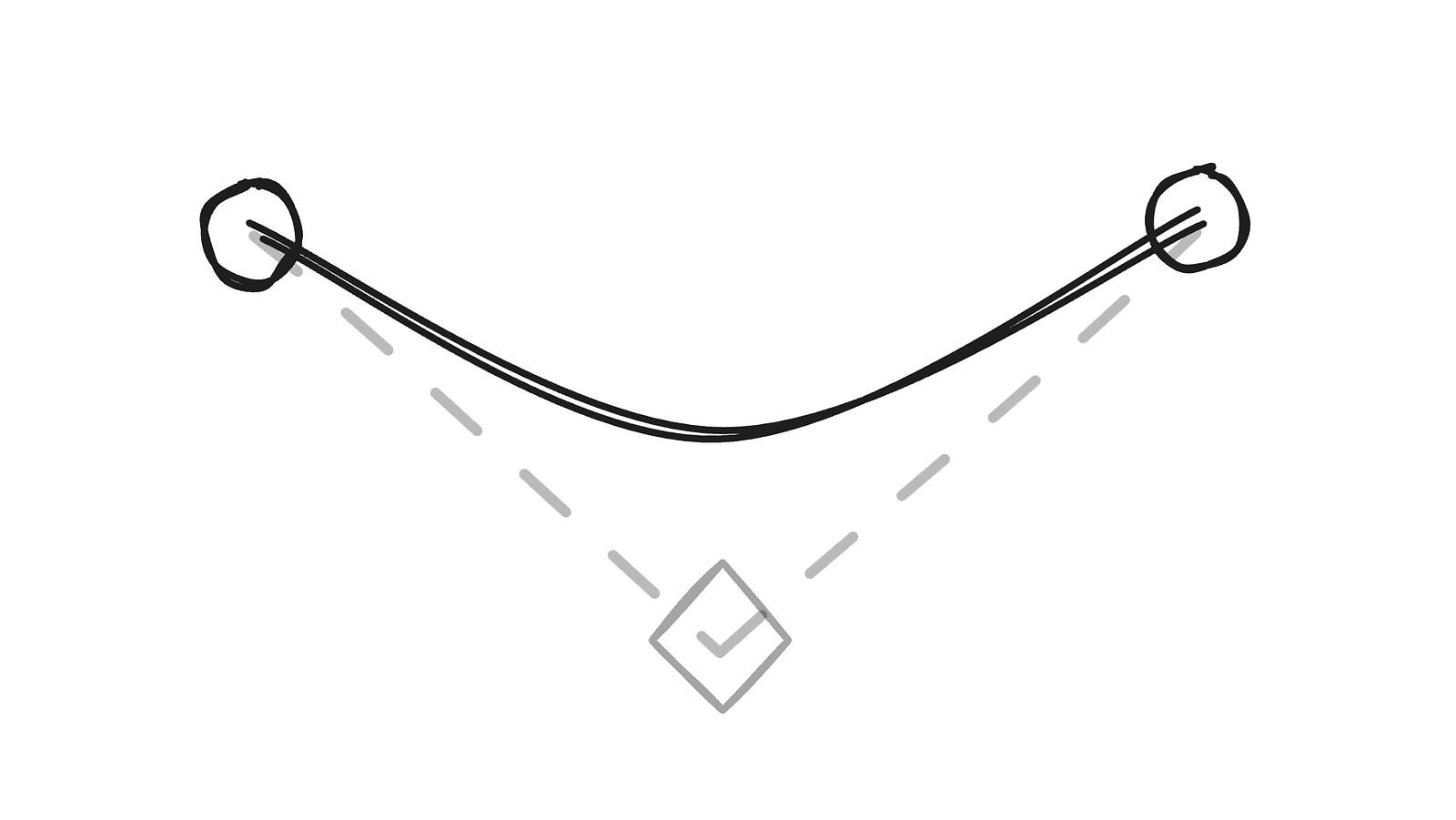
We already have a list of points for the slider, but we still need a third point for each segment to form the curves. This is where normals help. By using them, we can derive tangent lines, and the intersection of the tangents between two consecutive points gives us the control point for that segment.

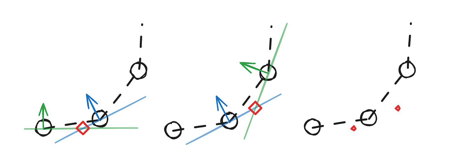
There’s one edge case we need to handle for this method to work reliably. When the tangents are parallel or nearly parallel, the control point either doesn’t exist (the lines never intersect) or ends up far from where it should be. Fortunately, this is easy to fix — in those cases, we simply place the control point at the midpoint between the two points.

Updating the GPU buffers

Now that we have all the necessary information, the final step is to prepare the data for use inside the shaders. The key idea here is that, for the data to be accessible on the GPU, we need to upload it into a buffer.

TypeGPU simplifies this process by providing schemas, so we don’t have to manually compute buffer sizes or memory layouts. Thanks to that, the entire GPU resource management for the slider’s data comes down to just a few straightforward steps:

class Slider {
  // Type declarations
  pointsReadonly: TgpuReadonly<d.WgslArray<d.Vec2f>>;
  controlPointsReadonly: TgpuReadonly<d.WgslArray<d.Vec2f>>;
  #normals: d.v2f[];
  #controlPoints: d.v2f[];

  constructor(...) {
    // Buffer creation
    this.#root.createReadonly(
      // Create a schema for n 2-component vectors
      d.arrayOf(d.vec2f, this.n),
      // The initial data
      this.#pos,
    );
    this.#root.createReadonly(
      d.arrayOf(d.vec2f, this.n - 1),
      this.#controlPoints,
    );
  }

  #updateGPUBuffer() {
    // Updating the buffers
    this.pointsReadonly.write(this.#pos);
    this.controlPointsReadonly.write(this.#controlPoints);
  }
}

After this step, it’s really up to us how we interpret this data in the rendering, so we can basically treat the entire engine as a black box.

The Rendering

To recap the simulation part, let’s quickly review the data we have and outline how we’ll use it.

We have:

• an ordered list of 2D points that define the slider’s path,
• an ordered list of control points computed from those points.

Looking at the reference render, the slider clearly doesn’t look strictly 2D — yet it only ever deforms along two axes. This means we can render it as a 2D line and simply extrude it along the third axis, placing the slider in 3D space even though the simulation itself is purely 2D.

We could build this with a mesh and deform it, and it would probably work — but looking at the reference, it’s clear we’ll also need advanced lighting, soft shadows, refraction, and some level of GI (global illumination) or AO (ambient occlusion). It’s all doable, but for a one‑off example the code would get complex quickly; we’d essentially be building a mini 3D engine from scratch. Fun, but not practical here.

Ray marching ends up being a much better fit:

• The slider needs to be perfectly smooth, which would be hard with a mesh unless we simulate a large number of points. With an SDF for the Bézier curve, we get a smooth surface “for free.”
• AO (ambient occlusion) is trivial with ray marching — because of SDFs, a single ray marched a few short steps is enough for good results.
• The background is easy to express as SDFs and extremely cheap to compute.

How does ray marching work?

There are many great resources that explain what ray marching is and how it works, so I will not go into much detail here. If you want an excellent reference, I recommend the articles by Inigo Quilez. For now, all we need to know is:

• we set a camera position (the camera will stay stationary, which is very convenient for us)
• we define a perspective projection that determines the direction of our rays
• for each pixel on the screen, we send a ray according to that direction — that ray determines what color we assign to the pixel

The ray checks its distance to the scene (the nearest object) and keeps moving forward until that distance is close enough to zero. At that point, it calculates the lighting for that position in space.

The background

For the ray to know how far it is from each element in the scene, we need to describe everything using signed distance fields. We’ll start by building the background. First, we’ll add a simple plane. We’ll define a function using TypeGPU, and by adding the `use gpu` directive at the top, the function becomes available inside a shader. We’ll also use the @typegpu/sdf helper package, which gives us SDF functions for common shapes (though you can implement them yourself from any reference — it’s just math).

const getMainSceneDist = (position: d.v3f) => {
  'use gpu';
  return sdf.sdPlane(position, d.vec3f(0, 1, 0), 0.06);
};

We defined a plane that spans the xz axis at y=0.06. It appears to cover the entire screen because the camera is tilted downward. That’s just an arbitrary choice — we could just as well keep the camera fixed and rotate the scene instead.

Now let’s create the cutout where the slider will sit. We’ll use a 2D rounded box and then extrude it into the third dimension.

const rectangleCutoutDist = (position: d.v2f) => {
  'use gpu';
  return sdf.sdRoundedBox2d(
    position,
    d.vec2f(1, 0.2), // width and height
    0.2, // the roundness factor
  );
};

const getMainSceneDist = (position: d.v3f) => {
  'use gpu';
  return sdf.opExtrudeY(
    position,
    rectangleCutoutDist(position.xz),
    0.01,
  );
}; 

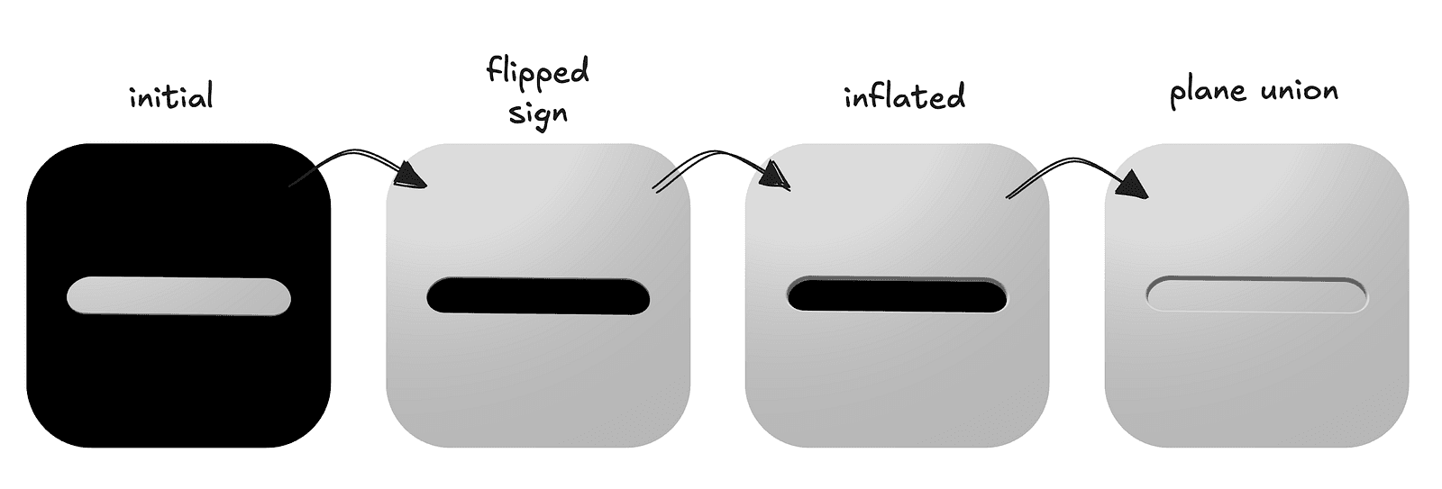
This will produce a slim rounded rectangle floating in space — but that’s not what we need, we actually need the opposite since it’s supposed to be a cutout. Thanks to the nature of SDFs, it’s as simple as flipping the sign on the rounded‑rectangle function.

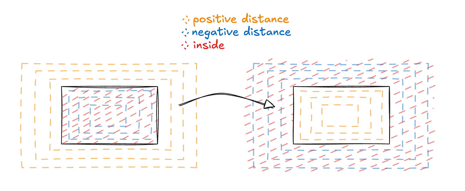
Our rectangle shape was already rounded, but this roundedness only applies to the 2D shape. The extrusion that brings it into the third dimension creates sharp edges, which do not match what we want. A solution for that is to use the inflation operation, which is very simple in nature — we basically subtract a flat amount from the distance. This means the shape will grow a bit, but all the sharp edges will get smoothed out.

After applying those operations, all that’s left is to patch the hole in the middle. We will do that using the union operation, which is basically taking the minimum of two distance fields. We add a plane at a small offset and make our scene the min of the two.

The final code for the background

const rectangleCutoutDist = (position: d.v2f) => {
  'use gpu';
  return sdf.sdRoundedBox2d(
    position,
    d.vec2f(1, 0.2),
    0.2,
  );
};

const getMainSceneDist = (position: d.v3f) => {
  'use gpu';
  return sdf.opUnion( // basically std.min
    sdf.sdPlane(position, d.vec3f(0, 1, 0), 0.06),
    sdf.opExtrudeY( // make it 3d
      position,
      -rectangleCutoutDist(position.xz), // sign flip
      0.01,
    ) - 0.02, // inflation
  );
};

You may have noticed that the background in the images is not just a uniform color but appears “lit.” There are many approaches to simulating lighting, but we will settle for one of the more popular and simple ones: the Phong lighting model. It is very well documented, and TypeGPU has a dedicated example for it.

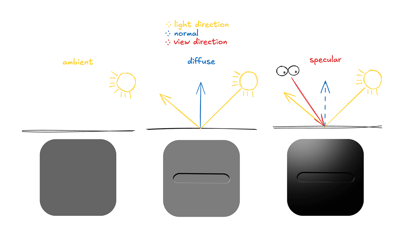
Basically, all we need is a light direction vector and a surface normal. The normal is a vector pointing away from the surface at a given point. With these, we can approximate lighting using three components:

• Ambient — the light that just is. It represents light that has bounced around the environment multiple times, without actually simulating those bounces.
• Diffuse — the light scattered by the material when it is hit by the light source. It depends on how directly the surface faces the light.
• Specular — the light that is directly reflected toward the observer, producing visible highlights on shiny surfaces.

If we look at the example code — cleaned up and reduced to just the core logic — it looks like this:

const calculateLighting = (
  hitPosition: d.v3f,
  normal: d.v3f,
  rayOrigin: d.v3f,
) => {
  'use gpu';
  // NOTE: This code operates under the assumption that light direction
  // is already normalized

  // the uniform contains the direction from the light, but for
  // the calculations we need the direction towards the light
  const lightDir = std.neg(lightUniform.$.direction);
  // we calculate the direction of the "eye" by taking the a vector from
  // the position the ray hit to the ray origin
  const viewDir = std.normalize(rayOrigin.sub(hitPosition));
  const reflectDir = std.reflect(std.neg(lightDir), normal);

  // ambient
  const ambientLight = AMBIENT_COLOR.mul(AMBIENT_INTENSITY);

  // diffuse
  const diffuseTerm = std.max(std.dot(normal, lightDir), 0.0);
  const diffuseLight = lightUniform.$.color
    .mul(diffuseTerm);

  // specular
  const specularTerm = std.max(std.dot(viewDir, reflectDir), 0) **
    SPECULAR_POWER;
  const specularLight = lightUniform.$.color.mul(specularTerm);

  // saturate(x) is basically max(0, min(1, x)))
  return std.saturate(diffuseLight.add(ambientLight).add(specularLight));
};

One important detail we’ve conveniently ignored so far is that we’ve been using normals as if we already had them — but we don’t.

In typical 3D models, normals are provided per vertex, along with position data and other attributes such as texture coordinates. The rendering pipeline simply interpolates them across the surface.

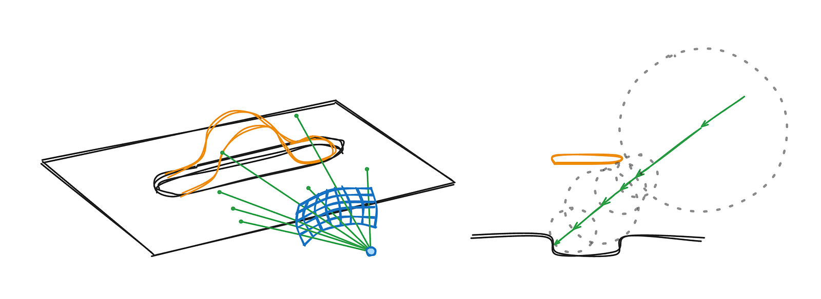
Here, however, we’re not working with a traditional mesh but rendering a signed distance field, which means there are no predefined vertices and no stored normals, so we need to compute the normal ourselves — fortunately, this is conceptually pretty easy, even if it can be computationally expensive.

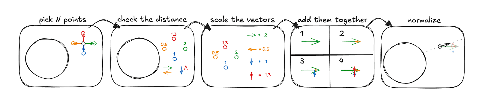
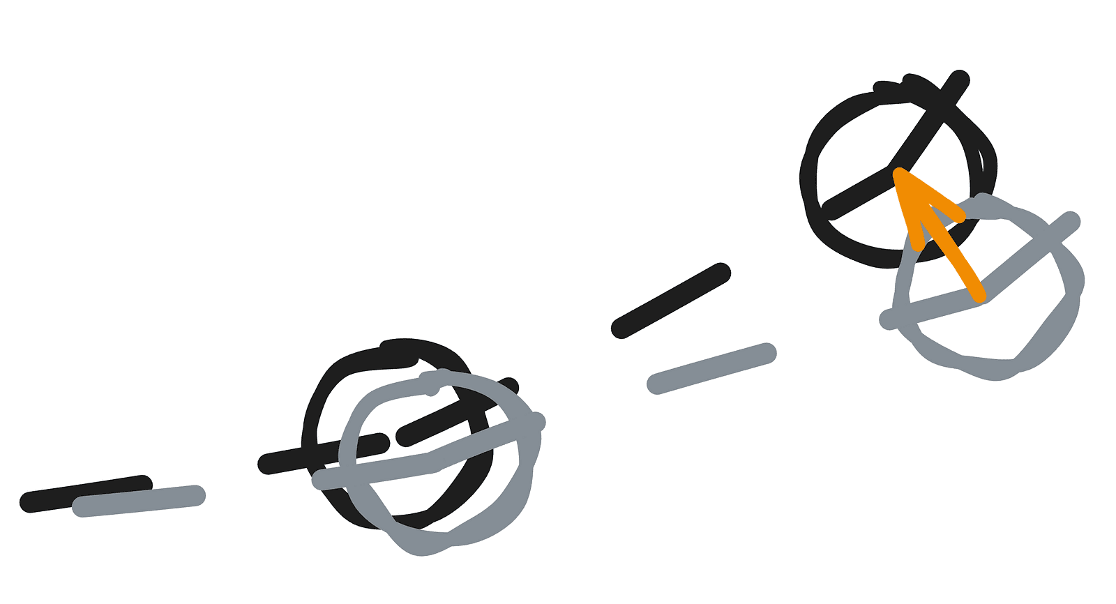
The example above computes a normal for an arbitrary point in 2D space, with greatly exaggerated distances for clarity. This process generalizes easily to 3D — you simply sample additional points and move the vectors into three-dimensional space. The important detail is that these sample points should be arranged symmetrically and contribute equally along each axis to produce a correct and unbiased normal. In the Jelly Slider, for performance reasons, we did not use the typical six-point normal approximation with two samples per axis. Instead, we used four points corresponding to the vertices of a regular tetrahedron. The underlying idea remains the same, and in practice, the results are not noticeably worse.

A key performance insight becomes obvious when we look at the main scene with normal visualization, where the absolute values of xyz components are mapped to rgb colors.

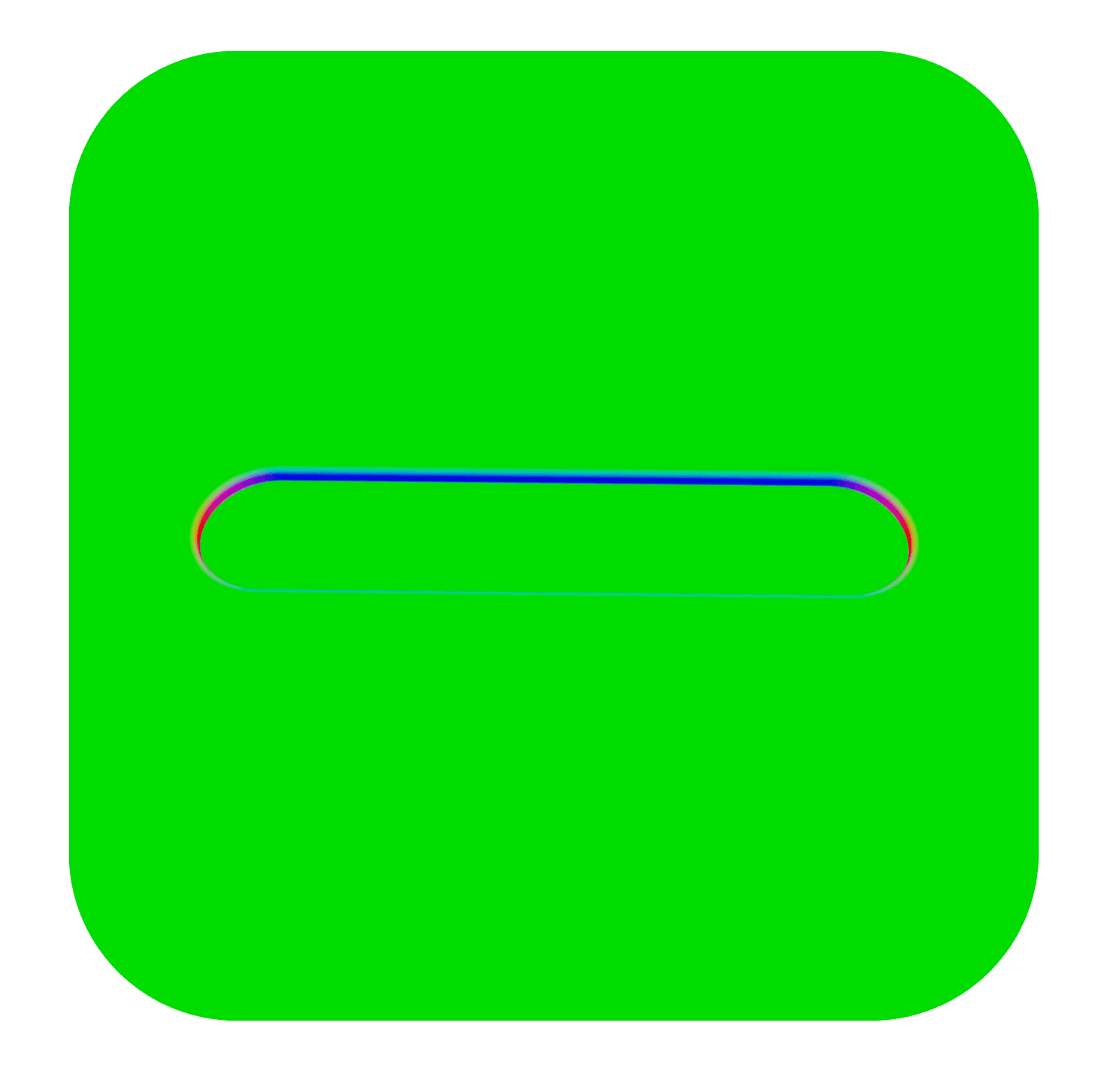
From the image above, it’s clear that a constant normal of [0, 1, 0] would already be a reasonable approximation for the entire scene — and for most of it, even a perfect one. The surface is largely flat and aligned in a single direction, so computing a full SDF-based normal at every point would be unnecessary overhead. That’s why, in the code, the normal calculation for the main scene is simplified to this:

const getNormalMain = (position: d.v3f) => {
  'use gpu';
  // check if we are outside the cutout area
  if (std.abs(position.z) > 0.22 || std.abs(position.x) > 1.02) {
    return d.vec3f(0, 1, 0);
  }
  // the full tetrahedral normal approximation
  return getNormalMainSdf(position, 0.0001);
};

The getNormalMainSdf function uses one of my favorite TypeGPU features: slots. Since there are multiple SDFs in the scene for which we may want to compute normals, we avoid duplicating code by implementing the tetrahedral normal approximation once and defining the actual SDF function as a slot. The slot represents any function that takes a position and returns a distance. This allows us to reuse the same normal computation logic across different parts of the scene by simply plugging in a different SDF implementation.

const getNormalFromSdf = tgpu.fn([d.vec3f, d.f32], d.vec3f)(
  (position, epsilon) => {
    'use gpu';
    // create the offset vectors (scaled by some small value)
    const offset1 = k.xyy * epsilon;
    const offset2 = k.yyx * epsilon;
    const offset3 = k.yxy * epsilon;
    const offset4 = k.xxx * epsilon;

    // scale the vectors by distance
    // sdfSlot.$ will be substituted with a function of choice later
    const sample1 = offset1 * sdfSlot.$(position + offset1);
    const sample2 = offset2 * sdfSlot.$(position + offset2);
    const sample3 = offset3 * sdfSlot.$(position + offset3);
    const sample4 = offset4 * sdfSlot.$(position + offset4);

    // create and normalize our normal from samples
    const gradient = sample1 + sample2 + sample3 + sample4;
    return std.normalize(gradient);
  },
);

// fill the slot with our main scene sdf (which we created earlier)
const getNormalMainSdf = getNormalFromSdf.with(sdfSlot, getMainSceneDist);

You may have noticed that the main scene — aside from currently lacking any jelly — looks somewhat flat. That’s because there are no shadows. While we could add them, shadow calculations in an SDF setup tend to be quite expensive, and in this case, we’ll rely on a couple of other tricks instead.

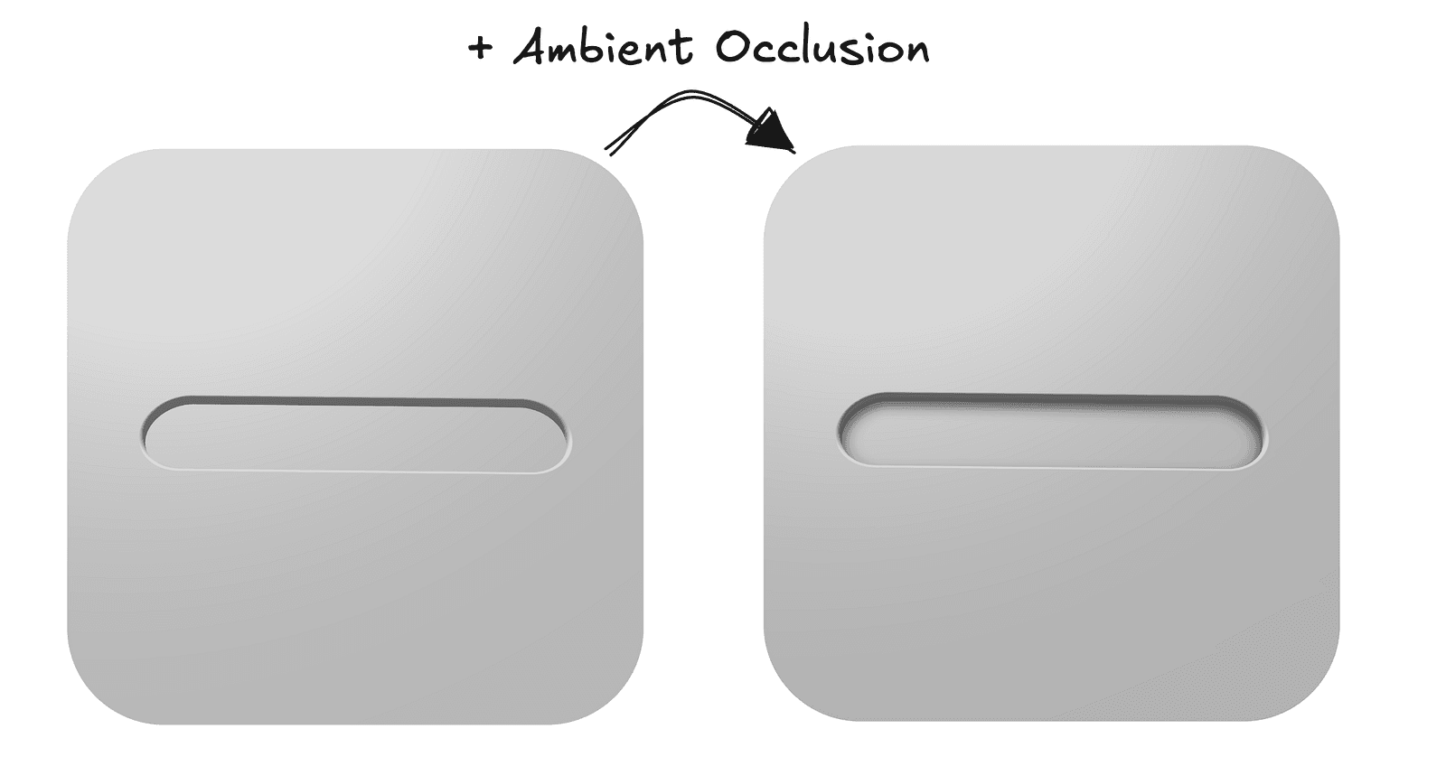
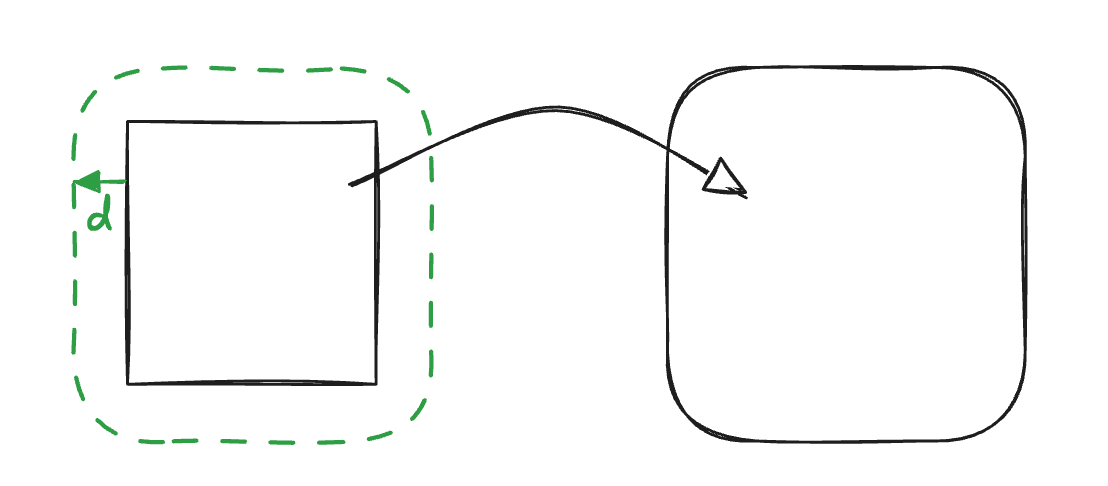
Ambient occlusion is a pretty common technique in computer graphics, but in the context of SDFs, I would argue it’s even more important due to the inherent nature of distance fields — specifically the fact that at any point in space, we already know the distance to the closest element of the scene, with no additional tricks required. Combined with the fact that we know how to calculate the normal at any point, we can fairly accurately estimate how occluded that point is, meaning how exposed it should be to ambient light.

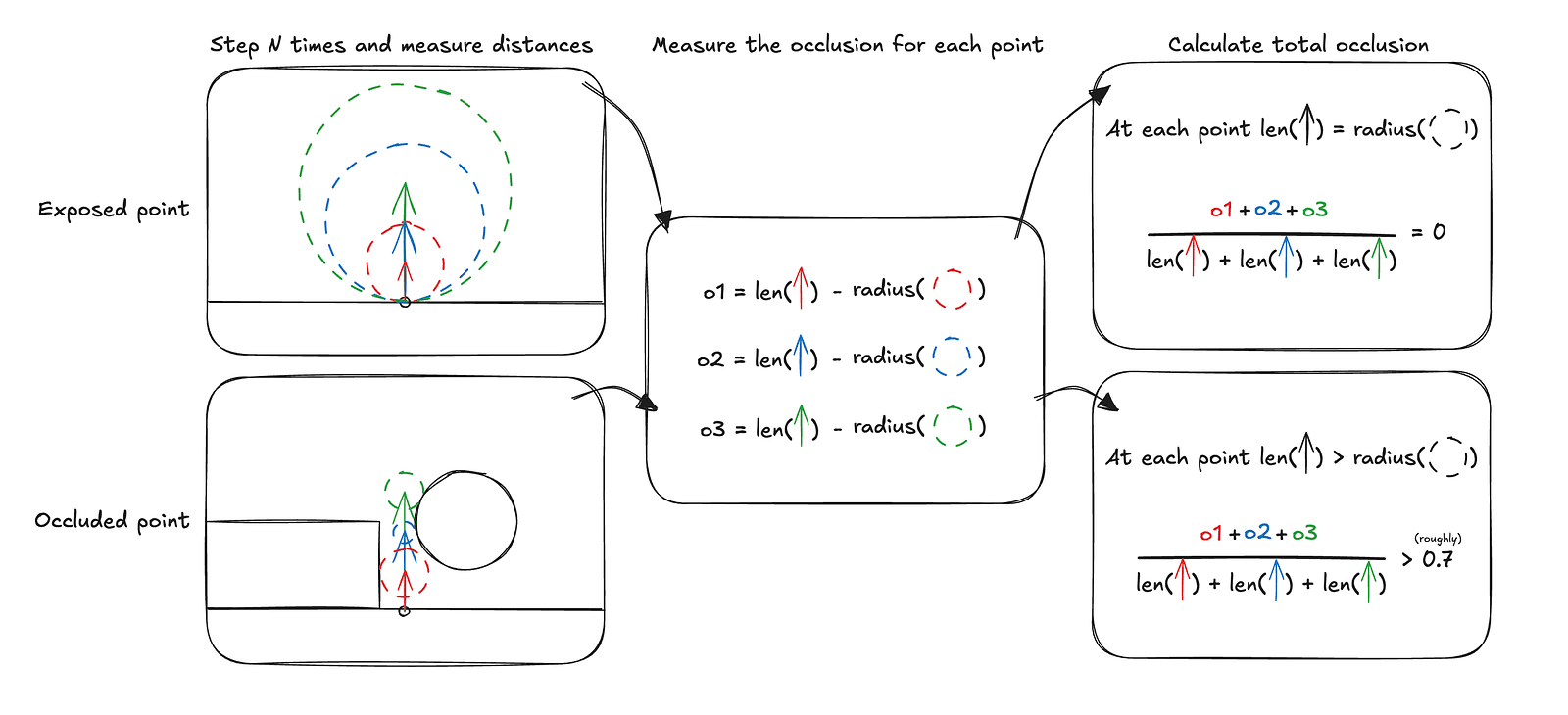
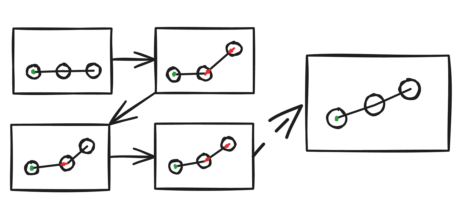
The diagram above illustrates how the occlusion calculation works over three steps, assuming each sample is treated equally, which in practice is usually not the case. In the Jelly Slider, we also use three steps, but each consecutive step contributes only half as much as the previous one.

const calculateAO = (position: d.v3f, normal: d.v3f) => {
  'use gpu';
  let totalOcclusion = d.f32(0);
  let totalWeight = d.f32(0);
  let sampleWeight = d.f32(1);

  for (let i = 1; i <= 3; i++) {
    const sampleHeight = (AO_RADIUS / 3) * d.f32(i);
    // get the point for AO sample
    const samplePosition = position + normal * sampleHeight;
    const distanceToSurface = getSceneDistForAO(samplePosition);

    // std.max is here to safeguard from numerical errors
    // distanceToSurface should never be > sampleHeight
    const occlusionContribution = std.max(0, sampleHeight - distanceToSurface);

    totalOcclusion += occlusionContribution * sampleWeight;
    totalWeight += sampleHeight * sampleWeight;
    sampleWeight *= 0.5;
  }

  const rawAO = 1.0 - totalOcclusion / totalWeight;
  return std.saturate(rawAO);
};

Since we already have the scene distance function and normal computation in place, the ambient occlusion implementation essentially comes down to performing three fixed ray marching steps along the normal and measuring the returned distances. While three steps are not free, they are still significantly cheaper than computing proper shadows.

It is important to stress that ambient occlusion is not a replacement for shadows. They model fundamentally different phenomena and only happen to produce a similar sense of depth in our very flat scene. The slider does use shadows, but they are not calculated using ray marching.

Jelly time

Now that we’ve established a solid foundation for rendering the scene, prepared the cutout for the jelly to sit in, and set up the simulation infrastructure, we’re ready to tackle arguably the most important part — actually rendering the slider itself.

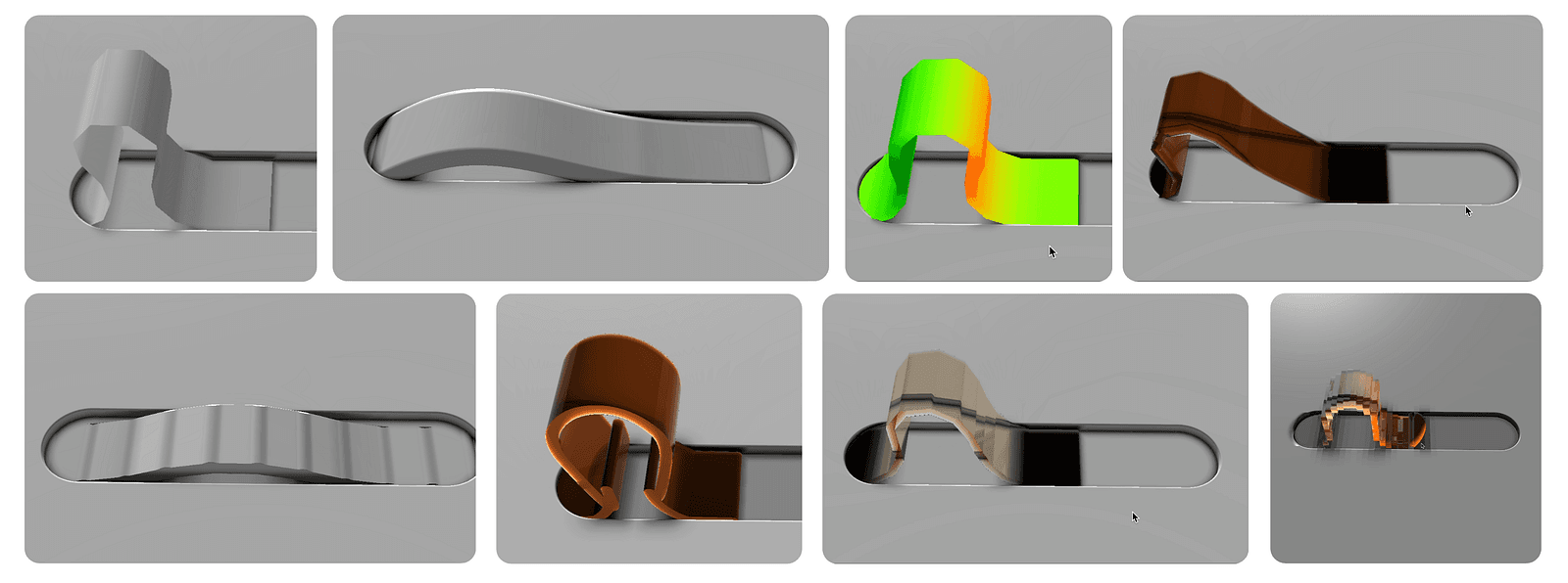
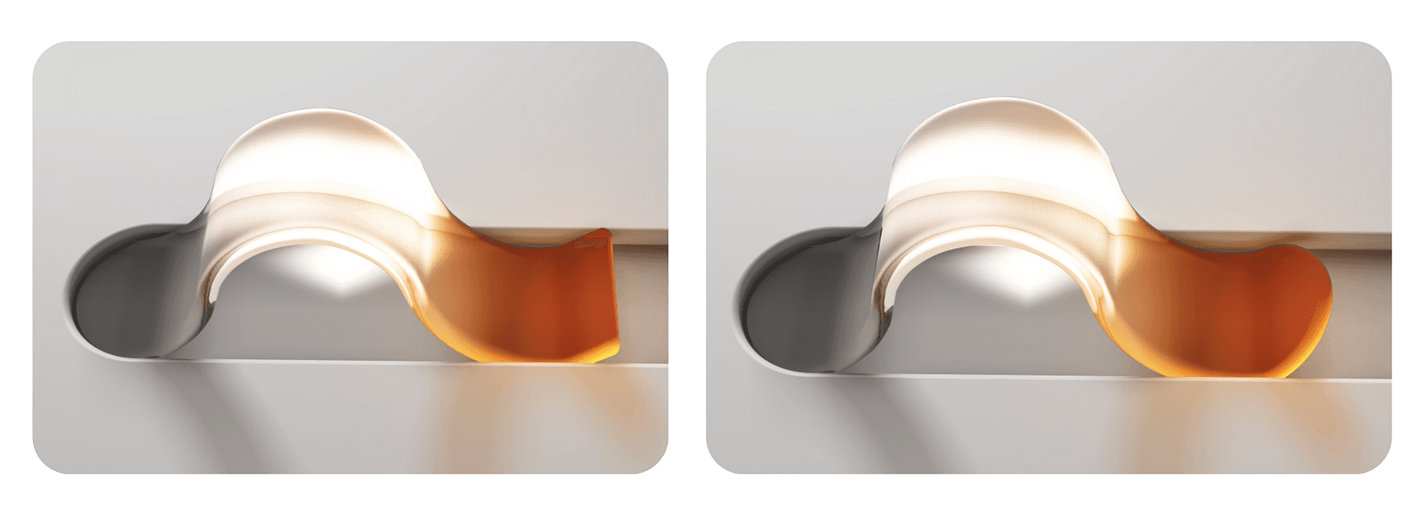
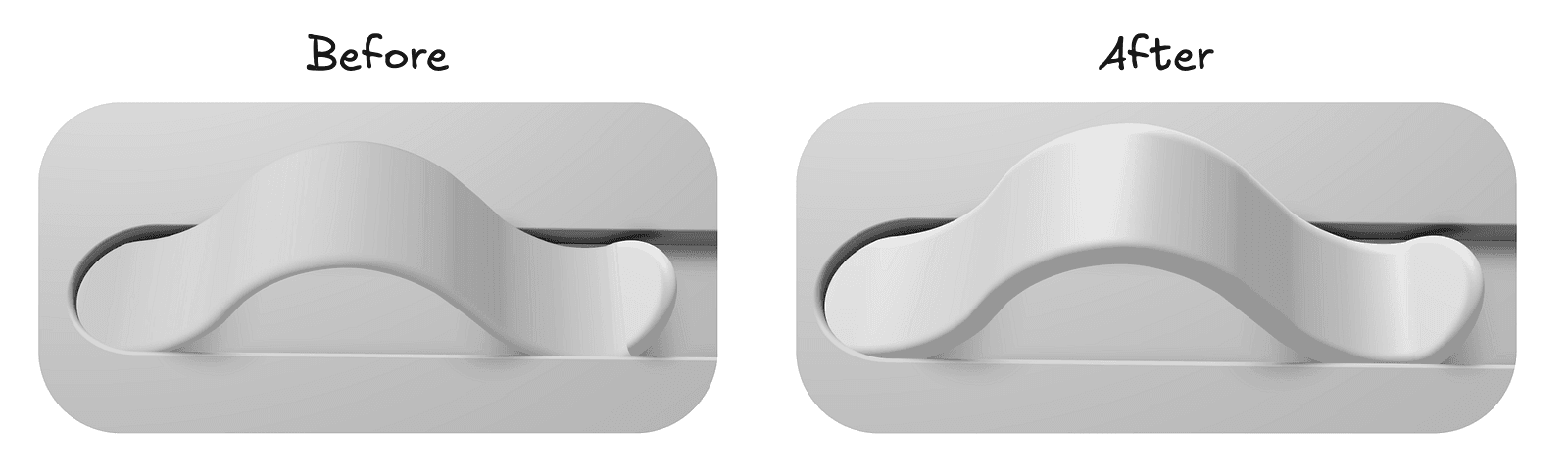
There are many feasible ways to get it on the screen — and quite a few were explored before settling on the final approach. Here are a couple of screenshots from different phases of experimentation:

There were two main challenges to solve, and for a long time, they felt mutually exclusive:

1. Appearance — we want the jelly to have a smooth surface and be as close to the reference in visual quality as possible. 2. Performance — the goal was to have it run smoothly even on mid to low-end phones.

The final approach took some iteration, but thankfully, a few things were working in our favor. The key idea was to pick the right primitive to construct the SDF from.

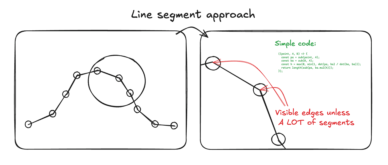
The initial attempt was to build it from a high number of points and line segments, since distances to those are very cheap to compute. This failed mainly because the physics simulation became the bottleneck at higher point counts. To achieve a convincing curve — especially when heavily bent — the number of required points was simply too high.

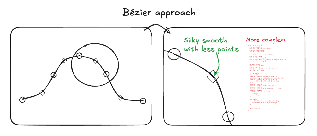
The second idea was to use Bézier curves (as you already know, this is the approach I ultimately landed on — just not immediately). Bézier curves give you very smooth visuals with a fraction of the control points, which is a huge advantage. The downside is that computing the distance to a Bézier curve is not trivial, both computationally and conceptually.

Calculating the distance to the Jelly Slider — which consists of 16 Bézier segments — for every ray is technically possible, but computationally far too expensive, even for mid-range desktops, let alone mobile devices.

To put this into perspective: in the best-case scenario for a 2K output at 2560 by 1440 pixels, we would need to solve 16 quadratic equations per ray, roughly 8 to 64 times per pixel per frame. Factoring that out gives approximately 1,887,436,800 quadratic equations to solve every single frame — clearly not a viable approach.

That said, this is a worst-case, brute-force estimate. There is, of course, a lot of room for optimization.

There are three main avenues we can explore in search of optimizations, though the first two are inherently connected.

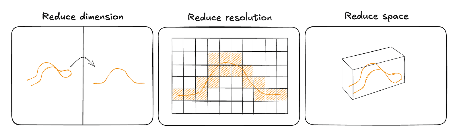
The key observation is that the slider is fundamentally two-dimensional. We only expand it into three dimensions using an SDF extrusion along the third axis, but the core information — the curvature — lives strictly in 2D.

This means we can precompute the expensive Bézier distance calculations once within a limited 2D region around the slider. Instead of solving quadratic equations at render time, we evaluate them ahead of time and store the results in a texture.

At runtime, this reduces the problem to a simple texture lookup. Not only is that dramatically cheaper than solving equations per pixel, but it also gives us interpolation for free*, allowing us to reduce the resolution while still maintaining smooth results.

* Of course, not completely free, but still cheaper than doing it by hand.

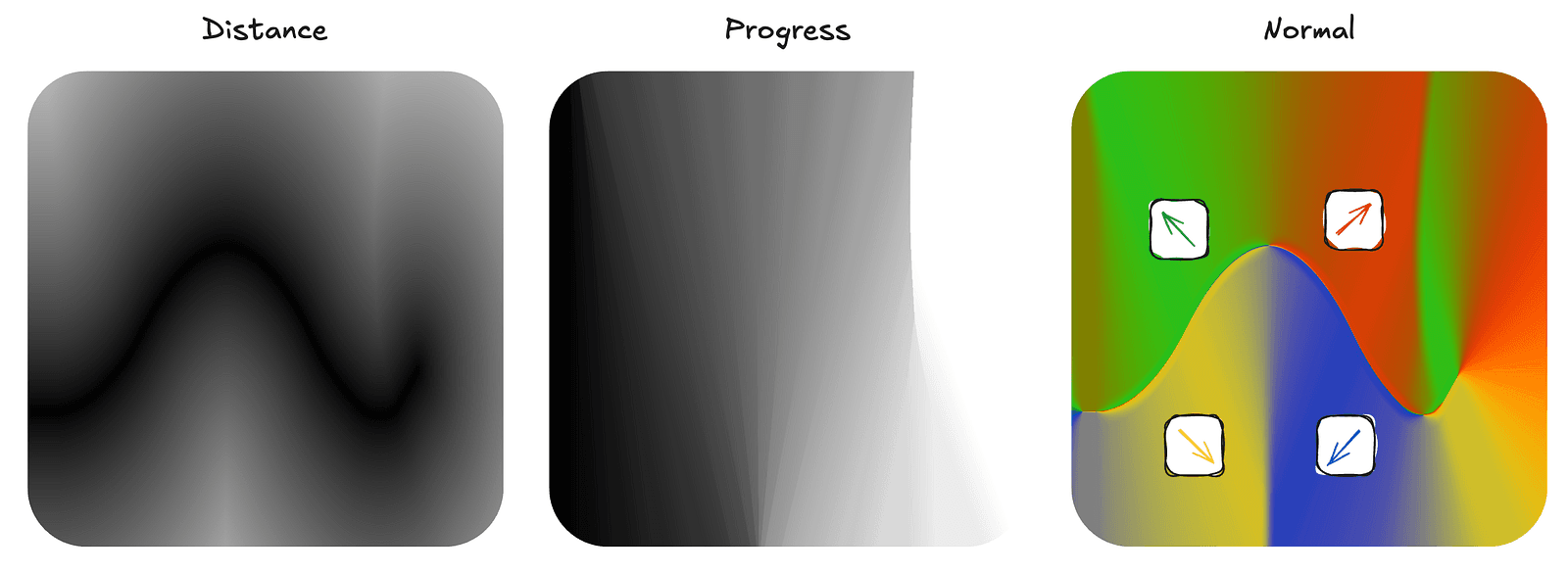
Since we’re already precomputing the data, we also store some useful auxiliary information to further reduce runtime work. Because the Jelly Slider is fundamentally 2D, we can pack quite a lot of data into a single pixel.

Each vec4f in the texture is laid out as follows:

• x — the raw distance to the nearest Bézier segment
• y — the progress value, meaning how far along the slider we are, normalized to the 0–1 range
• z and w — the precomputed normal at that point

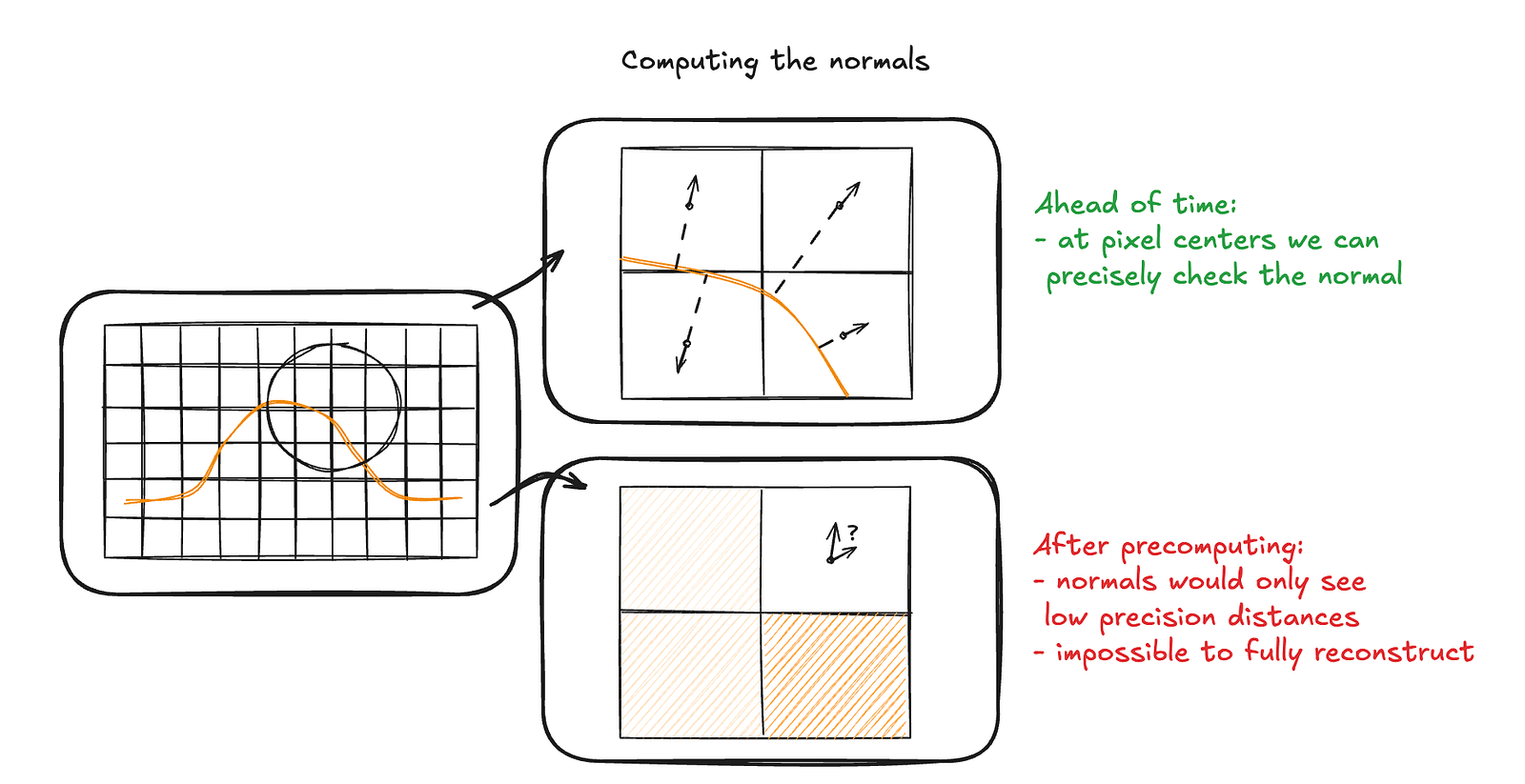
By storing the normal directly, we avoid additional texture samples to reconstruct it, and we also retain the full effective resolution of the data. Reconstructing normals from quantized distance values would introduce additional error and visibly degrade the result. Precomputing and storing them explicitly keeps both the shader logic simpler and the visual quality higher.

Great, so we now have a 2D texture containing all the information we need — but how do we actually use it?

One of the great properties of SDFs is that you can evaluate them anywhere in space by simply passing in a position and the primitive parameters. That convenience no longer fully applies here. The texture has limited bounds, so we need to know when to sample it and how to map world space positions to texture space.

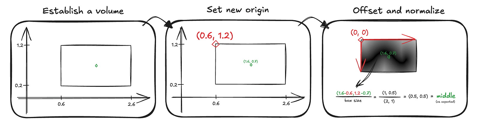
This is where the third optimization helps — and conveniently solves this problem as well. We define a bounding volume in world space that fully contains the slider.

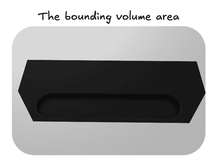
This helps in two ways.

First, ray–box intersection tests are simple and computationally cheap, so we can quickly determine whether a ray even has a chance of hitting the slider.

Second, once we transform a point into the box’s local space — effectively redefining the coordinate system with one corner of the box as the origin — we regain the convenient SDF-like behavior. A normalized position inside this box space directly maps to texture coordinates, which tells us exactly where to sample the precomputed distance field to retrieve the jelly slider data.

The code that converts our encoded data into a meaningful shader variable looks like this:

const sdInflatedPolyline2D = (p: d.v2f) => {
  'use gpu';
  const bbox = getSliderBbox();

  // checking where to sample the texture as shown above
  const uv = d.vec2f(
    (p.x - bbox.left) / (bbox.right - bbox.left),
    (bbox.top - p.y) / (bbox.top - bbox.bottom),
  );
  const clampedUV = std.saturate(uv);

  // decoding the slider info
  const sampledColor = std.textureSampleLevel(bezierTexture.$, filteringSampler.$, clampedUV, 0);
  const segUnsigned = sampledColor.x;
  const progress = sampledColor.y;
  const normal = sampledColor.zw;

  return LineInfo({
    t: progress,
    distance: segUnsigned,
    normal: normal,
  });
};

This function computes the distance to the slider for a given 2D point. On its own, that would make the slider infinite along the third dimension, so we add a helper that extrudes the shape into 3D. This both bounds the volume and adds an end cap, implemented as a half-pie SDF computed from the last two points of the slider.

const sliderSdf3D = (position: d.v3f) => {
  'use gpu';
  const poly2D = sdInflatedPolyline2D(position.xy);

  let finalDist = d.f32(0);
  if (poly2D.t > 0.94) {
    finalDist = cap3D(position);
  } else {
    const body = sdf.opExtrudeZ(
      position,
      poly2D.distance,
      LINE_HALF_THICK
    ) - LINE_RADIUS;
    finalDist = body;
  }

  return LineInfo({
    t: poly2D.t,
    distance: finalDist,
    normal: poly2D.normal,
  });
};

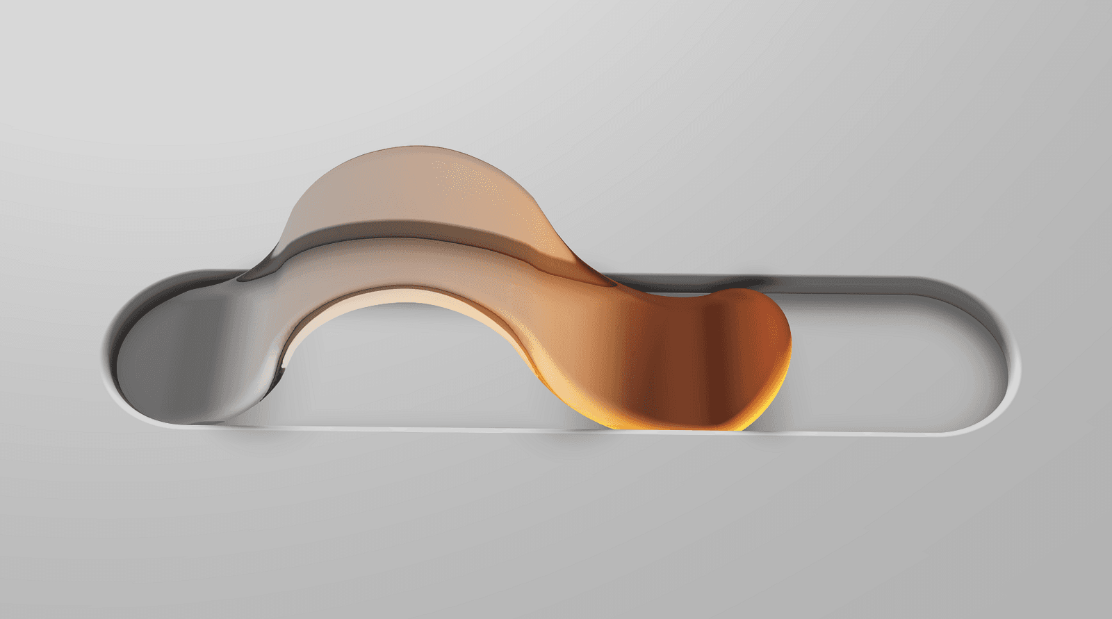
Actually, the fully rendered preview in the image above is a bit premature. At this stage, we only have the raw information about the slider, so it actually looks more like this:

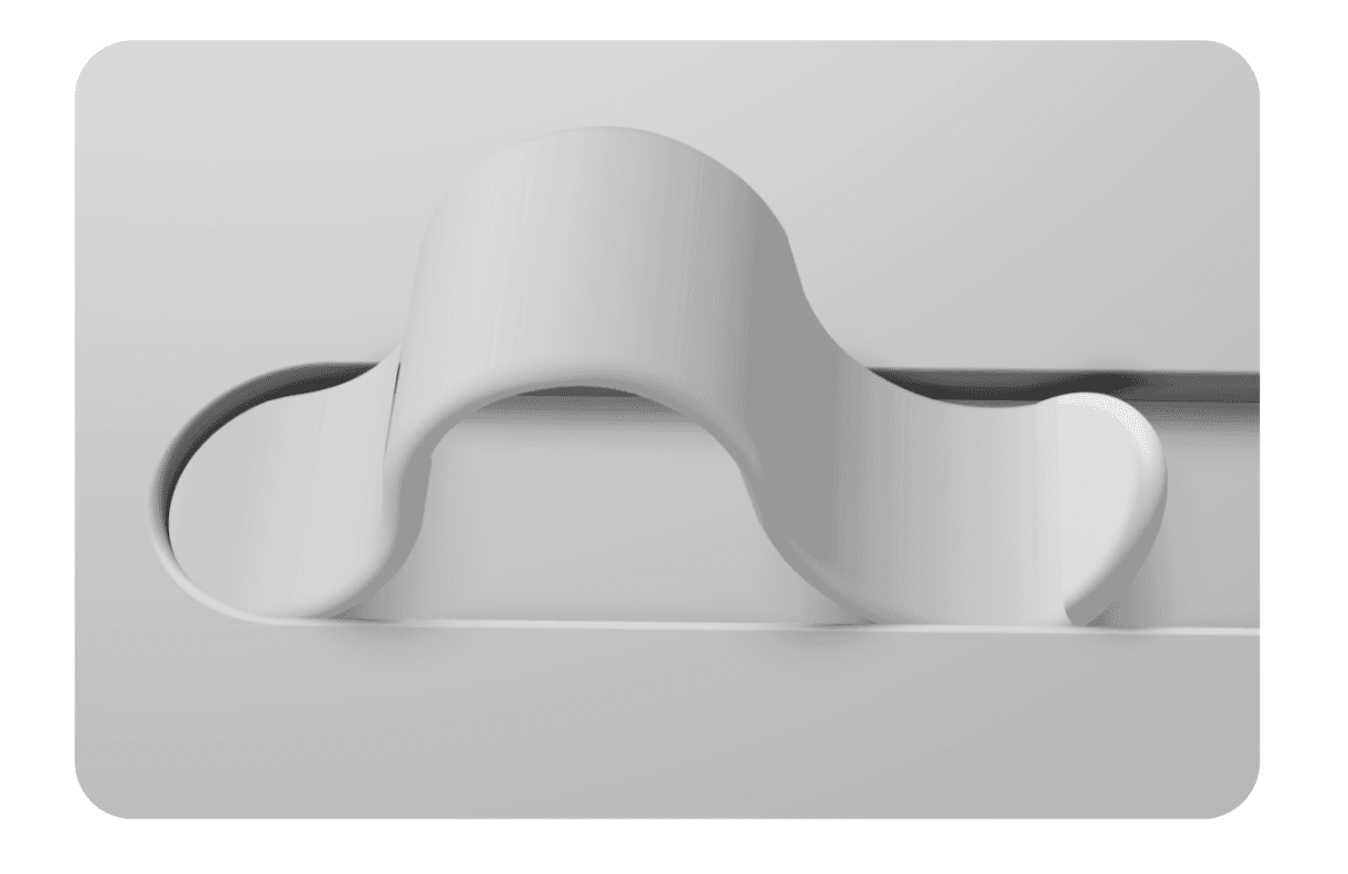
Since our current lighting logic only knows how to render the ground, it treats rays that hit the slider the same way. Another issue that becomes immediately obvious near the cap area is that linear interpolation is not enough to produce believable lighting for the slider. We will need some additional smoothing logic along the edges.

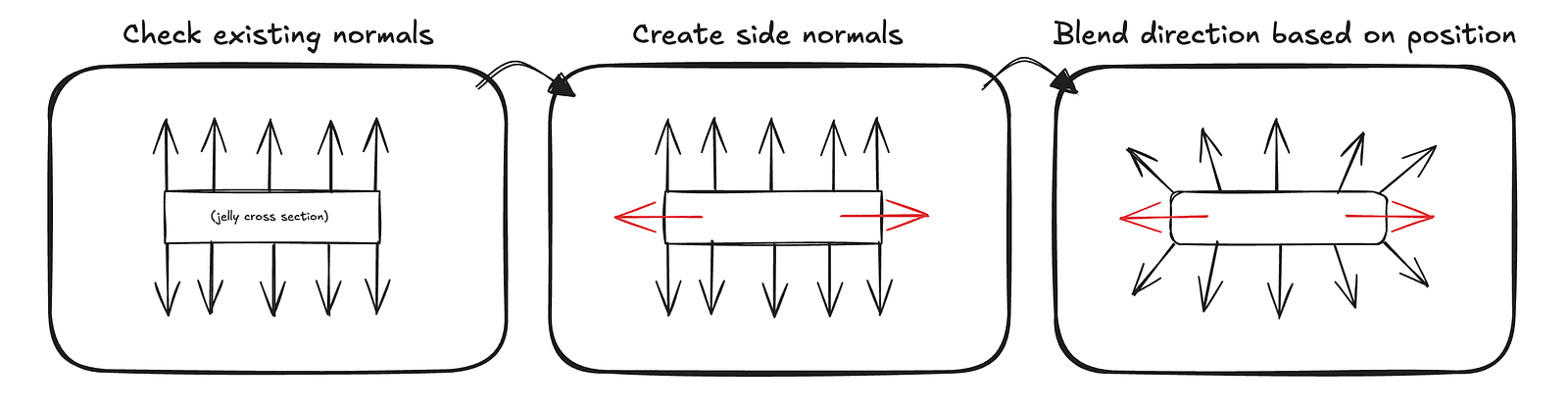
Our slider is fixed along the x-axis, so creating rounded normals for the edges to better simulate the smooth shape is fairly straightforward. We check the z position of the hit and create a vector pointing in the z direction, vec3f(0, 0, 1)with the same sign as the z position. Then, using the slider width, which is conveniently constant, we blend between the interpolated normal read from the texture and this z vector.

This requires some trial and error with the blending ratios to get the smoothing right, but it ultimately allows us to match the curvature of the cap almost perfectly.

Now the only core thing left is to make the slider transparent. That might sound scary and complicated, but we actually already have most of the pieces in place. The main missing part is the refraction logic so the light bends realistically inside the slider. Once we determine where the refracted ray should travel, we can simply march along that direction while ignoring the slider itself.

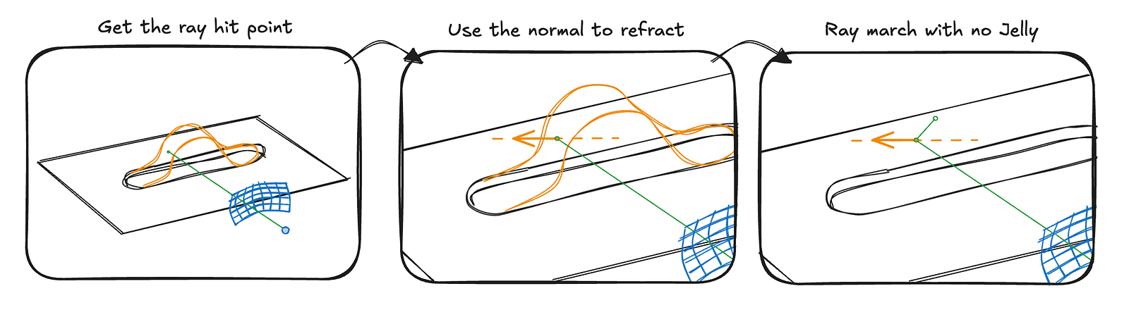
In code, this becomes a simple conditional branch in the ray marching loop. rayMarchNoJelly is a small ray marching routine that runs for six steps, which is more than enough to produce convincing refractions. If nothing is hit after six steps, we simply take the closest point reached so far, which turns out to be a good enough approximation.

if (hitInfo.distance < SURF_DIST && hitInfo.objectType === ObjectType.SLIDER) {
  const hitPosition = rayOrigin + rayDirection * distanceFromOrigin;

  const N = getNormal(hitPosition, hitInfo);

  const eta = 1 / JELLY_IOR;
  const refrDir = std.refract(rayDirection, N, eta);

  const env = rayMarchNoJelly(hitPosition, refrDir);
  const progress = hitInfo.t;
  const jellyColor = jellyColorUniform.$;

  const scatterTint = jellyColor.rgb * 1.5;
  const absorb = (1 - jellyColor.rgb) * 20;

  const T = beerLambert(absorb * (progress ** 2), 0.08);

  const lightDir = std.neg(lightUniform.$.direction);

  const forward = std.max(0, std.dot(lightDir, refrDir));
  const scatter = scatterTint * (JELLY_SCATTER * forward * progress ** 3);
  const refractedColor = env * T + scatter;

  return d.vec4f(refractedColor, 1);
}

The code is simplified by assuming a constant thickness, which turns out to be good enough. We could ray march inside the volume or derive a formula to calculate how much jelly the light travels through, but that would either be expensive or time-consuming for a detail that is barely noticeable.

Putting everything we discussed in this article together, we get:

Not quite a 1:1 match with the original example, but close enough without diving into too much additional detail. Everything that is missing can be derived from what we have covered so far. The shadow is simply the slider texture projected onto the plane, the subtle glow is derived from the slider distance, the highlight in the middle is entirely hard-coded, and the text rendered on the ground is just an image.

The code is public, and I encourage you to explore and experiment with it. With what you know now, you will probably be able to quickly identify the remaining tricks used in the implementation.

Thank you for reading to the end :) I hope this article was detailed enough to convey some useful techniques and spark interest in graphics programming while still staying engaging. If you have any questions, feel free to reach out on the TypeGPU Discord server, where I am often around, or contact me directly on X.